CityHop

Case Study

About

CityHop is a fast-growing ride-sharing app operating in over 50 cities. The company's success hinges on its ability to make smart, data-driven decisions for dynamic pricing, driver incentives, and operational efficiency. The platform generates millions of data points daily from trips, payments, and user activity.

The Challenge

The current data infrastructure, built quickly for launch, is now a major bottleneck. It relies on slow, hourly batch scripts and a rigid SQL database. This system cannot provide timely insights, struggles with complex analytical queries, and is failing under the weight of increasing data volume. The business is flying blind on critical performance metrics.

Solution

The primary objective is to write the production-level SQL queries necessary to answer the following list of critical business questions

Daily Active Riders

This query is fundamental for understanding daily user engagement, a key performance indicator for CityHop. It calculates the number of unique riders active on any given day. To achieve this, the CAST(trip_timestamp AS DATE) function standardizes the data by removing the time component from the trip_timestamp column, allowing all trips to be grouped by the calendar day. The core logic lies in the COUNT(DISTINCT rider_id) aggregate function. This counts the unique rider identifiers within each daily group, which is crucial for ensuring a rider who takes multiple trips in one day is only counted once. Finally, the GROUP BY and ORDER BY clauses structure the output.

Daily Revenue Growth

This query calculates the day-over-day percentage growth in total fare revenue, a vital metric for tracking business momentum. It uses a Common Table Expression (CTE) named DailyRevenue to first aggregate the total fare for each day. A second CTE, RevenueWithLag, then utilizes the LAG window function to create a new column, previous_day_fare, containing the total fare from the preceding day.

This setup is crucial for comparing consecutive days. Finally, the main query calculates the growth percentage using the standard formula. A CASE statement is included to handle the very first day of data, preventing a division-by-zero error and ensuring the query is robust.

Top Profitable Routes

This SQL query identifies the top 5 most profitable travel routes in the CityHop database by calculating the total fare amount collected on each route. It follows a structured approach using Common Table Expressions (CTEs):

RouteFares CTE: It first groups data in the Trips table by start_loc and end_loc, representing a unique route. For each route, it computes the sum of all fares, giving the total earnings (total_route_fare) per route.

RankedRoutes CTE: It ranks all the routes using the DENSE_RANK() window function, ordered by total_route_fare in descending order. This means the route with the highest earnings gets rank 1, the second-highest gets rank 2, and so on. DENSE_RANK ensures that if multiple routes have the same fare, they get the same rank without skipping numbers.

Final Selection: It filters and displays only those routes that fall within the top 5 ranks, ensuring ties are included. The result is ordered by total_route_fare in descending order, showing the most profitable routes at the top.

This analysis helps businesses optimize operations by focusing on high-revenue routes.

Rolling Revenue Comparison

This SQL query analyzes 30-day rolling fare revenue trends in the CityHop database, helping identify revenue growth or decline over time. It uses Common Table Expressions (CTEs) to compare the current 30-day revenue window with the one immediately before it:

DailyRevenue CTE: Aggregates total fare (daily_fare) for each day by casting trip_timestamp to a DATE. This provides daily revenue data across the timeline.

RollingRevenue CTE: Calculates the rolling 30-day sum of fares using the SUM() window function. The clause ROWS BETWEEN 29 PRECEDING AND CURRENT ROW ensures that for each date, the sum of that day and the previous 29 days is computed—giving a moving 30-day revenue total.

Final Selection: Uses LAG() to compare the current 30-day rolling fare with the same figure from 30 days earlier (previous_30_day_fare). This helps evaluate whether the recent 30-day window performed better or worse than the previous one.

The result highlights revenue shifts over time, aiding business teams in detecting trends, seasonality, or anomalies in fare collection.

Top Drivers by Zone

This SQL query identifies the top 3 highest-earning drivers in each city zone within the CityHop database by calculating their total fare earnings and ranking them within their respective zones.

It begins by joining the Drivers and Trips tables to compute the total fares earned by each driver, grouping the results by driver ID, name, and home zone. This gives a summary of how much each driver has earned overall.

Next, it ranks drivers within each home_zone using the DENSE_RANK() window function, ordered by total fares in descending order. This ensures that drivers with the highest earnings in each zone are ranked at the top. Finally, it filters the result to include only the top 3 ranked drivers in each zone, presenting their names, total fares earned, and rank.

The output is sorted by home_zone and fare amount, helping the business understand who their top-performing drivers are in each geographic area. This insight can support decisions around rewards, retention strategies, or targeted performance improvement.

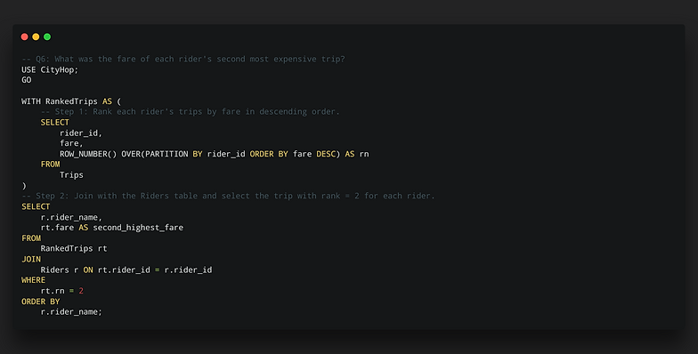
Second Highest Fare

This query identifies the second most expensive trip for each rider. It uses a Common Table Expression (CTE) named RankedTrips to first assign a rank to every trip. The ROW_NUMBER() window function is partitioned by rider_id, which means it restarts the ranking for each individual rider. Within each partition, trips are ordered by fare in descending order, so the most expensive trip gets rank 1, the next gets rank 2, and so on. The final SELECT statement then joins this CTE with the Riders table to get the rider's name and filters the results to only include rows where the rank (rn) is exactly 2, effectively isolating each rider's second-highest fare. This method correctly handles all riders, only returning a result for those who have taken at least two trips.

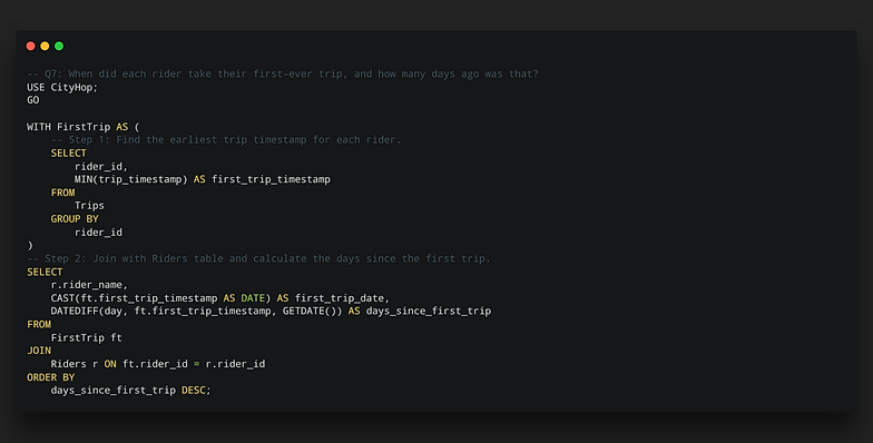
Rider First Trip

This query is designed to determine each rider's first-ever trip date and subsequently calculate their tenure with CityHop in days. It provides valuable information for cohort analysis and understanding customer loyalty. The logic begins with a Common Table Expression (CTE) named FirstTrip, which efficiently finds the earliest (minimum) trip_timestamp for each unique rider_id by using the MIN() aggregate function and grouping the results. This initial step isolates the exact moment of each rider's first interaction with the service.

The main SELECT statement then joins this CTE with the Riders table to associate the first trip data with the corresponding rider's name. It formats the timestamp into a clean date for readability and uses the DATEDIFF() function to calculate the precise number of days between that first trip and the current date (GETDATE()), providing a clear measure of customer longevity.

Quick Plus Subscribers

This query identifies "quick adopters" - riders who subscribed to CityHop Plus shortly after their first experience with the service. This is a key metric for gauging the immediate value perception of the premium offering.

The query first establishes the date of each rider's inaugural trip using a Common Table Expression (CTE) named FirstTrip, which finds the minimum trip timestamp for each user. This CTE is then joined back to the main Riders table, which contains the plus_sub_date. The WHERE clause is crucial: it filters for riders who have a non-null subscription date and then uses the DATEDIFF function to calculate the interval between their first trip and their subscription. By filtering this interval to be 7 days or less, the query precisely isolates the target group of early-subscribing, high-engagement customers, providing valuable data for marketing and product teams.

Cumulative Ride Types

This query tracks how a rider's usage of different services evolves over time. It calculates a running count of the unique ride types ('Standard', 'Premium', 'Pool') for each rider. This is a powerful way to measure customer exploration and adoption of higher-value services.

The query uses a COUNT(DISTINCT ride_type) window function. The PARTITION BY t.rider_id clause is essential, as it isolates the calculation for each rider independently. The ORDER BY t.trip_timestamp clause arranges each rider's trips chronologically, so the function counts the unique ride types from their very first trip up to the current one, showing their service discovery journey trip-by-trip.

Consistent Rider Analysis

This query identifies "power riders" who demonstrate consistent engagement by taking three or more trips in a single week. The analysis focuses on recent activity by dynamically defining a two-month window, starting from the latest trip date recorded in the dataset. This ensures the query remains relevant as new data is added.

Inside a Common Table Expression (CTE), trips are grouped by each rider and the specific week they occurred in. The HAVING clause then acts as a filter, retaining only those rider-week combinations that meet the "3 or more trips" threshold. Finally, the query joins back to the Riders table to retrieve the names and uses DISTINCT to present a clean, unique list of these highly active users. This insight is critical for designing loyalty programs and understanding the habits of the most valuable customer segment.

Consistent Rider Analysis

Rider Ranking

The first CTE, RiderQuarterlyTrips, calculates the total_trips for each rider within every unique quarter and year. This is achieved by joining the

Trips and Riders tables, then grouping the data by rider ID, name, year, and quarter, and finally counting the trips.

The second CTE, RankedRiderQuarterlyTrips, then takes these quarterly trip counts and applies a ranking. It uses the ROW_NUMBER() window function, partitioning the data by year and quarter and ordering it by total_trips in descending order, to assign a sequential rank to each rider within that specific quarter.

The final SELECT statement retrieves the rider's name, year, quarter, total trips, and their calculated quarterly rank, ordered chronologically and by rank for clarity.